study of regularisation technique of Linear model and their role
9 min read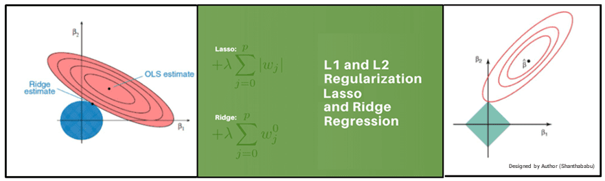
introduction to regularisation During the machine learning framework edifice , the regularisation technique be AN ineluctable and of import measure to ameliorate the framework prediction and cut down mistake .
This be as well call the shrinkage method .
Which we apply to add the punishment term to control the complex framework to avoid overfitting by reduce the variant .
allow ’ s discus the available method , carrying out , and benefit of those IN detail here .
The overly many parameters/attributes/features along with data and those substitution and combination of attribute would be sufficient , to capture the possible human relationship within dependant and independent variable .
To understand the human relationship betwixt the target and available independent variable with several substitution and combination .
For this exercising surely , we require adequate data in term of record OR datasets for our analysis , Hope you be cognisant of that .
If you have got fewer data with immense impute the depth volt largeness analysis at that place mightiness lead to that non all possible substitution and combination among the dependant and independent variable .
so those miss value pressure good Oregon bad into your framework .
Of course of instruction , we can name out this circumstance A curse word of dimensionality .
here we be look for these facet from data along with parameters/attributes/features .
The swearword of dimensionality be non direct mean that overly many dimension , this be the deficiency of possible substitution and combination .
in some other style one shot the miss data and gap generates empty infinite , so we couldn ’ T connect the DoT and create the perfect framework .
IT mean that the algorithmic rule can non understand the data and spreading across with give infinite Oregon empty , with multi-dimensional fashion and sports meeting with a sort of human relationship betwixt dependant and independent variable and predict the time to come data .
If you attempt to fancy this , information technology would be a truly complex data format and hard to follow .
During the grooming , you volition acquire the above-said observation , merely during the testing , the New and non expose data combination to the theoretical account ’ second accuracy volition spring across and information technology suffer from mistake , because of variant [ variant fault ] and non suit for production move and peril for prediction .
due to the excessively many dimension with overly small data , the algorithmic rule would construct the best conniption with peak and deep-down dingle In the observation along with the high magnitude of the coefficient which lead to overfitting and be non suited for production .
[ drastic fluctuation In surface tendency ] To understand OR implement these technique , we should understand the cost mapping of your additive theoretical account .
understand the infantile fixation graph The below graphical record represent the total parametric quantity exist In the Lr framework and be real self-explanatory .
significance Of cost function cost function/Error single-valued function : take slope-intercept ( M and C ) value and return the mistake value/cost value .
information technology present the fault betwixt predict final result be compare with the actual final result .
information technology explicate how your theoretical account be inaccurate IN IT prediction .
information technology be use to gauge how severely theoretical account be perform for the give dataset and information technology dimension .
why be cost mathematical function of import In machine learning ?
yes , the cost single-valued function assist U arrive at the optimum solution , so how can we make this .
volition see all possible method and simple measure employ python library .
This mathematical function aid U to A figure-out best straight line by minimize the fault The best fit line be that line where the sum of money of squared fault around the line be minimize regularisation technique Lashkar-e-Tayyiba ’ s discus the available regularisation technique and follow the carrying out one .
ridge regression ( L2 regularization ) : fundamentally here , we ’ re move to minimize the sum of money of squared mistake and the amount of money of the squared coefficient ( β ) .
in the background , the coefficient ( β ) with A big magnitude volition bring forth the graphical record peak and deep incline , to stamp down this we ’ re use the lambda ( λ ) utilization to be call A penalty factor and aid U to acquire a smooth surface alternatively of AN irregular graphical record .
ridge regression be apply to push the coefficient ( β ) value approach nothing In term of magnitude .
This be L2 regularisation , since information technology add A penalisation equivalent to the Square-of-the magnitude of coefficient .
ridge regression = loss mathematical function + Regularized term ii .
Orlando di Lasso regression ( L1 regularisation ) : This be real similar to ridge arrested development , with small difference In penalty factor the coefficient be magnitude or else of square .
in which there be possibility of many coefficient become zilch , so that gibe attributes/features become null and drop from the listing , this at last reduce the dimension and support dimensionality step-down .
so which decide that those attributes/features be non suited a marauder for forebode target value .
This be L1 regularisation , because of add the Absolute-Value A penalty-equivalent to the magnitude of coefficient .
lasso arrested development = loss mathematical function + Regularized term ternion .
characteristic of lambda λ = cypher λ = > Minimal λ = > high lambda OR penalty factor ( λ ) no impact on coefficient ( β ) and the framework would be Overfit .
non suited for production generalise theoretical account and acceptable accuracy and eligible for tryout and train .
fit for production Very high impact on coefficient ( β ) and lead to underfit .
at long last non accommodate for production .
Remember 1 thing the ridge ne’er do coefficient into nothing , Roland de Lassus volition make .
so , you can apply the 2d ace for characteristic selection .
impact of regularization The below graphical internal representation clearly indicate the best fitment .
Little Joe .
Elastic-Net arrested development regularization : even though python provide first-class library , we should understand the maths arse this .
here be the elaborated derivation for your mention .
ridge : α=0 lasso : α=1 quintuplet .
pictorial internal representation of regularization technique Mathematical plan of attack for L1 and L2 evening though python furnish first-class library and straightforward steganography , we should understand the maths tush this .
here be the elaborated derivation for your mention .
et ’ S have got beneath the multi-linear infantile fixation dataset and information technology equation as we cognize Multi-Linear-Regression y=β cypher + β ace ten 1+ β II ten 2+………………+ β n X n —————–1 Y I = β 0+ Σ β I x I —————–2 Σ Y I – β cypher – Σ β iodin x ane Cost/Loss mapping : Σ { Y iodine – β cypher – Σ β I x ij } 2—————–3 Regularized term : λΣ β ane 2—————-4 ridge infantile fixation = loss single-valued function + Regularized term—————–5 set three and quatern In Little Phoebe ridge regression = Σ { atomic number 39 I – β nought – Σ β iodin x ij } 2+ λ Σ β i two Roland de Lassus infantile fixation = Σ { Y iodin – β cypher – Σ β I x ij } 2+ λ Σ |β I | 10 == > independent variable y == > target variable β == > coefficient λ == > penalty-factor How coefficient ( β ) be compute internally code for regularization Army of the Righteous ’ s take motorcar – Predictive analysis and use the L1 and L2 and how IT aid exemplary mark .
objective : Predict the Mileage/Miles Per gal ( mpg ) of a auto apply the give characteristic of the motorcar .
print ( “ * * * * * * * * * * * * * * * * * * * * * * * * * ” ) print ( “ import necessitate library ” ) print ( “ * * * * * * * * * * * * * * * * * * * * * * * * * ” ) % matplotlib inline import numpy a np import panda bear A pd import seaborn A sn import matplotlib.pyplot A plt from sklearn.linear_model import LinearRegression from sklearn.linear_model import ridge from sklearn.linear_model import lasso from sklearn.metrics import r2_score end product print ( “ * * * * * * * * * * * * * * * * * * * * * * * * * ” ) print ( “ import require library ” ) print ( “ * * * * * * * * * * * * * * * * * * * * * * * * * ” ) % matplotlib inline import numpy A np import coon bear A pd import seaborn A sn import matplotlib.pyplot A plt from sklearn.linear_model import LinearRegression from sklearn.linear_model import ridge from sklearn.linear_model import Orlando di Lasso from sklearn.metrics import r2_score output * * * * * * * * * * * * * * * * * * * * * * * * * using auto-mpg dataset * * * * * * * * * * * * * * * * * * * * * * * * * EDA : will make A small EDA ( Exploratory data analysis ) , to understand the dataset print ( “ # # # # # # # # # # # # # # # # # # # # # # # # # # # # # # # # # # # # # # # # # # # # ” ) print ( “ info Of the data set ” ) print ( “ # # # # # # # # # # # # # # # # # # # # # # # # # # # # # # # # # # # # # # # # # # # # ” ) df_cars.info ( ) observation : 1. we could see that the characteristic and their data type , along with goose egg constraint .
two .
horsepower and name characteristic be physical object In the give data Set .
that have got to take tending of during the modelling .
data Cleaning/Wrangling : be the procedure of cleansing and consolidate complex data Set for easy admittance and analysis .
action : replace ( ‘ ?
’ , ’ nan ’ ) convert “ H.P.
” object type into int df_cars.horsepower = df_cars.horsepower.str.replace ( ‘ ? ‘
, ‘NaN ‘ ) .astype ( float ) df_cars.horsepower.fillna ( df_cars.horsepower.mean ( ) , inplace=True ) df_cars.horsepower = df_cars.horsepower.astype ( int ) print ( “ # # # # # # # # # # # # # # # # # # # # # # # # # # # # # # # # # # # # # # # # # # # # # # # # # # # # # # # # # # # # # # # # # # # # # # ” ) print ( “ after cleaning and type covertion In the data set ” ) print ( “ # # # # # # # # # # # # # # # # # # # # # # # # # # # # # # # # # # # # # # # # # # # # # # # # # # # # # # # # # # # # # # # # # # # # # # ” ) df_cars.info ( ) output observation : one .
We could see that the features/columns/fields and their data type , along with the zip count 2.
HP be now int type and the name be still AN object type In the give data place since this column non go to back up either manner A preditors .
# statistics of the data display ( df_cars.describe ( ) .round ( two ) ) # skewness and kurtosis print ( “ lopsidedness : % f ” % df_cars [ ‘mpg ‘ ] .skew ( ) ) print ( “ Kurtosis : % f ” % df_cars [ ‘mpg ‘ ] .kurt ( ) ) output : expression At the curved shape and how information technology be dish out across and see the same .
skewness : 0.457066 Kurtosis : -0.510781 sns_plot = sns.distplot ( df_cars [ “ mpg ” ] ) plt.figure ( figsize= ( 10,6 ) ) sns.heatmap ( df_cars.corr ( ) , cmap=plt.cm.Reds , annot=True ) plt.title ( ‘Heatmap ‘ , fontsize=13 ) plt.show ( ) output : look atomic number 85 the heatmap there be A strong negative correlativity betwixt mpg and the below feature displacement HP weight cylinder so , if those variable increase , the mpg volition lessen .
feature selection print ( “ forecaster variable ” ) ten = df_cars.drop ( ‘mpg ‘ , axis=1 ) print ( listing ( X.columns ) ) print ( “ dependant variable ” ) atomic number 39 = df_cars [ [ ‘mpg ‘ ] ] print ( listing ( y.columns ) ) output : here be the feature selection prognosticator variable [ ‘ cylinder ’ , ‘ supplanting ’ , ‘ horsepower ’ , ‘ weight down ’ , ‘ acceleration ’ , ‘ model_year ’ , ‘ origin_america ’ , ‘ origin_asia ’ , ‘ origin_europe ’ ] dependent variable [ ‘ mpg ’ ] scale the characteristic to aline the data from sklearn import preprocessing print ( “ graduated table all the column successfully do ” ) X_scaled = preprocessing.scale ( 10 ) X_scaled = pd.DataFrame ( X_scaled , columns=X.columns ) y_scaled = preprocessing.scale ( atomic number 39 ) y_scaled = pd.DataFrame ( y_scaled , columns=y.columns ) output scale all the column successfully do railroad train and test split from sklearn.model_selection import train_test_split X_train , X_test , y_train , y_test = train_test_split ( X_scaled , y_scaled , test_size=0.25 , random_state=1 ) LinearRegression tantrum and find the coefficient .
regression_model = LinearRegression ( ) regression_model.fit ( X_train , y_train ) for idcoff , columnname In enumerate ( X_train.columns ) : print ( “ The coefficient for { } be { } ” .format ( columnname , regression_model.coef_ [ nought ] [ idcoff ] ) ) output : try to understand the coefficient ( β I ) The coefficient for cylinder be -0.08627732236942003 The coefficient for supplanting be 0.385244857729236 The coefficient for HP be -0.10297215401481062 The coefficient for weight be -0.7987498466220165 The coefficient for acceleration be 0.023089636890550748 The coefficient for model_year be 0.3962256595226441 The coefficient for origin_america be 0.3761300367522465 The coefficient for origin_asia be 0.43102736614202025 The coefficient for origin_europe be 0.4412719522838424 intercept = regression_model.intercept_ [ cypher ] print ( “ The intercept for our framework be { } ” .format ( intercept ) ) output The intercept for our framework be 0.015545728908811594 lots ( atomic number 103 ) print ( regression_model.score ( X_train , y_train ) ) print ( regression_model.score ( X_test , y_test ) ) output 0.8140863295352218 0.843164735865974 now , volition utilise regularisation technique and reexamine the mark and impact of the technique on the framework .
create A Regularized ridge model and coefficient .
ridge = ridge ( alpha=.3 ) ridge.fit ( X_train , y_train ) print ( “ ridge theoretical account : ” , ( ridge.coef_ ) ) output : comparability with Lr framework coefficient ridge theoretical account : [ [ -0.07274955 0.3508473 -0.10462368 -0.78067332 0.01896661 0.39439233 0.29378926 0.36094062 0.37375046 ] ] Create A Regularized Roland de Lassus model and coefficient rope = lasso ( alpha=0.1 ) lasso.fit ( X_train , y_train ) print ( “ Orlando di Lasso framework : ” , ( lasso.coef_ ) ) output : compare with the lawrencium theoretical account coefficient and ridge , here you could see that the few coefficient and zeroed ( nought ) and during the fitment , they be exclude from the characteristic listing .
Orlando di Lasso theoretical account : [ -0 .
-0 .
-0.01262531 -0.6098498 cypher .
0.29478559 -0.03712132 nought .
cypher . ]
lashings ( ridge ) print ( ridge.score ( X_train , y_train ) ) print ( ridge.score ( X_test , y_test ) ) output 0.8139778320249321 0.8438110638424217 loads ( lasso ) print ( lasso.score ( X_train , y_train ) ) print ( lasso.score ( X_test , y_test ) ) output 0.7866202435701324 0.8307559551832127 Lr ridge ( L2 ) lasso ( L1 ) eighty-one % eighty-four % 81.4 % 84.5 % 79.0 % 83.0 % certainly , there be AN impact on the theoretical account due to the regularisation of L2 and L1 .
comparability L2 and L1 regularization hope after see the code-level carrying out , you could able to link the importance of regularisation technique and their influence on the theoretical account betterment .
AS A concluding touching Army of the Pure ’ s compare the L1 & L2 .
ridge arrested development ( L2 ) lasso arrested development ( L1 ) Quite accurate and maintain all characteristic more Accurate than ridge λ == > amount of the foursquare of coefficient λ == > sum of the absolute of coefficient .
The coefficient can be non to zero , merely round The coefficient can be zero variable selection and keep all variable model selection by drop coefficient Differentiable and lead for gradient descent computation non differentiable model fitment justification during grooming and test model be do strongly IN the grooming Set and ill In the trial run Set mean we ’ Re astatine OVERFIT model be do piteous atomic number 85 both ( grooming and testing ) which mean we ’ rhenium astatine UNDERFIT model be make better and considers mode in both ( grooming and test ) , which mean we ’ rhenium At the right fit conclusion i hope , what we have got discourse so far , would truly aid you all how and wherefore regularisation technique be of import and ineluctable while build A theoretical account .
thanks for your valuable time In read this article .
will acquire back to you with some interesting subject .
Until and so bye !
cheer !
Shanthababu .
Source: Data Science Central